What Is the Expected Move?
The Expected Move (EM) is the options market’s consensus estimate of how far an underlying asset will move over a specific time period. It is expressed as a dollar amount (or percentage) and represents a one standard deviation (1-SD) price range — meaning there is approximately a 68% probability that the stock will remain within the expected move bounds by expiration.
If AAPL is trading at $200 and the weekly expected move is $6, the market is saying: “There is a 68% chance that AAPL will be between $194 and $206 by Friday’s close.” Extending to two standard deviations (2-SD), the 95% probability range is $188–$212. The remaining 5% encompasses tail events — moves larger than the market anticipated.
The expected move is not a prediction of direction. It says nothing about whether AAPL will go up or down. It quantifies magnitude — how far, not which way. This makes it the foundation for non-directional strategies (iron condors, straddles) and a critical input for directional strategies (determining whether your price target is within or beyond the expected range). The EM is the practical output of implied volatility — every change in IV recalculates the range in real time.
The Expected Move Formula
The mathematical formula for expected move derives directly from implied volatility:
Expected Move = Stock Price × IV × √(DTE / 365)
Where: Stock Price = current price, IV = annualized implied volatility (decimal form), DTE = days to expiration.
This formula works because implied volatility is expressed as an annualized standard deviation. To convert from annual to any shorter time period, you multiply by the square root of the time fraction. This square-root scaling is a fundamental property of volatility under the assumption of normally distributed returns — the same principle that makes the HV formula use √252 as its annualization factor.
Worked Examples
| Stock | Price | IV | DTE | 1-SD EM ($) | 1-SD Range | 2-SD Range (95%) |
|---|---|---|---|---|---|---|
| AAPL | $200 | 25% | 7 | $6.93 | $193.07 – $206.93 | $186.14 – $213.86 |
| AAPL | $200 | 25% | 30 | $14.33 | $185.67 – $214.33 | $171.34 – $228.66 |
| SPX | 5,800 | 18% | 1 (0DTE) | $54.62 | 5,745 – 5,855 | 5,691 – 5,909 |
| TSLA | $250 | 55% | 7 | $19.04 | $230.96 – $269.04 | $211.92 – $288.08 |
| TSLA | $250 | 55% | 30 | $39.40 | $210.60 – $289.40 | $171.20 – $328.80 |
Notice how the expected move does not scale linearly with time. Doubling the DTE from 7 to 14 days increases the expected move by only ~41% (not 100%) due to the square-root relationship. This has profound implications for strategy selection: shorter-dated options provide tighter expected move bounds, which increases the probability of success for credit strategies but also means less time for the underlying to reach a directional target.
The √T Scaling Rule
Quick mental math shortcuts for converting between time periods:
- Daily to Weekly: Multiply daily EM by √5 ≈ 2.24
- Weekly to Monthly: Multiply weekly EM by √4.3 ≈ 2.07
- Daily to Monthly: Multiply daily EM by √21 ≈ 4.58
- VIX to Daily SPX move: VIX ÷ √252 ≈ VIX ÷ 15.87
The Straddle Shortcut: Reading EM from the Chain
You do not need to calculate the expected move formula manually. The options chain provides it directly through the at-the-money straddle price:
Expected Move ≈ ATM Straddle Price
The at-the-money straddle (call + put at the same strike) is priced to reflect the market’s expected move for that expiration. If the ATM straddle costs $8, the market expects approximately ±$8 from the current price. For a more precise estimate, multiply the straddle price by 0.85 — this corrects for the straddle’s slight overpricing relative to the true 1-SD boundary caused by put skew.
This shortcut works because the Black-Scholes framework prices the ATM straddle at approximately 0.80 × σ × √T × S (where σ is IV, T is time, S is spot price). The straddle price naturally embeds the expected move calculation. Professional traders on exchange floors have used this shortcut for decades — it is the fastest way to gauge expected move without any calculation.
For earnings plays, the straddle shortcut is especially valuable. The ATM straddle for the expiration immediately after earnings directly prices the market’s expected earnings move. If AAPL reports Tuesday after close and the Friday straddle costs $12, the market expects a ±$12 (±6%) earnings move. If you believe the move will be larger, buy the straddle. If smaller, sell it. The full earnings EM framework — including historical move comparison and IV crush mechanics — is covered in Section 7 below.
Why the Expected Move Matters for Every Strategy
The expected move is not just a theoretical concept — it directly determines the profitability framework for every options strategy type:
| Strategy Type | Relationship to EM | Profit Condition |
|---|---|---|
| Iron Condor / Credit Spread | Short strikes placed at or beyond EM bounds | Profit if stock stays within the EM range |
| Long Straddle / Strangle | Cost equals approximately the EM | Profit if stock moves beyond the EM range in either direction |
| Debit Spread (directional) | Target strike relative to EM boundary | Profit if stock reaches target; EM defines whether the target is “within expectations” |
| Butterfly | Center strike = price target; wings at ±EM provides natural width | Profit if stock closes near center strike at expiration |
| Covered Call / Cash-Secured Put | Short strike beyond 1-SD EM = ~84% probability of keeping premium | Profit if stock stays below (call) or above (put) the short strike |
The key insight: the expected move defines the boundary between “probable” and “improbable” outcomes. Strategies that profit from probable outcomes (stock stays within EM) have high win rates but capped gains. Strategies that profit from improbable outcomes (stock exceeds EM) have lower win rates but outsized gains. Choosing between them depends on your volatility view — specifically whether current IV Rank and the IV–HV spread favor selling or buying premium.
Expected Move for Strike Selection
The most practical daily application of expected move is strike selection for credit strategies. The expected move bounds map directly to Delta-based strike selection:
| Strike Placement | Approx. Delta | Probability OTM | Best For |
|---|---|---|---|
| At 1-SD EM boundary | ~0.16 | ~84% | Standard credit spread / iron condor short strikes |
| At 1.5-SD | ~0.07 | ~93% | Wide iron condors; conservative premium selling |
| At 2-SD EM boundary | ~0.025 | ~97.5% | Protective wings; tail-risk hedges |
| Inside 1-SD (closer to ATM) | 0.20–0.40 | 60–80% | Aggressive credit collection; higher premium but higher risk |
The professional approach to iron condor construction: place short strikes at the 1-SD EM boundary (Delta ~0.16 each side) and buy protective wings 1–3 strikes further out. This creates a position with approximately 68% probability of both sides expiring OTM, collecting roughly 1/3 of the spread width in premium — the time-tested edge for systematic income strategies.
For directional debit spreads, the expected move answers the critical question: “Is my price target realistic?” If your analysis says AAPL will reach $210 in two weeks, but the expected move says the 2-week 1-SD range is only $194–$206, your target is beyond the expected range — possible, but the options market considers it a less than 16% probability event. Either your analysis has genuine edge over the market, or your target is too ambitious. The EM boundary is the market’s verdict on that question. For a complete framework on how to score the structural conviction behind any given EM boundary, see the Strike Wall Analysis framework — it explains which EM-boundary strikes have active dealer defense and which are structurally empty.
Expected Move vs. GEX Strike Walls: When Probability Meets Mechanics
The expected move is a statistical boundary — it says where price is likely to stay given current implied volatility, based on a probability distribution. A GEX strike wall is a mechanical boundary — it exists because dealers have live hedging obligations at that strike that force them to buy or sell the underlying as price approaches. These two frameworks answer different questions, but when they converge on the same strike, the structural conviction of that level compounds significantly.
Three Convergence Scenarios
| Scenario | EM Boundary | Strike Wall Score | Structural Interpretation | Trading Implication |
|---|---|---|---|---|
| Double Conviction | 1-SD boundary | 3–4 / 4 (live wall) | Probabilistic range AND mechanical dealer defense at the same strike | Highest-conviction short-strike placement for credit spreads; dealers mechanically defend, EM defines probability |
| Statistical Only | 1-SD boundary | 1 / 4 (OI only, no gamma) | EM boundary looks like support on paper — but the wall is “dead”: no active dealer hedging below it | Treat as a probability reference, not a mechanical floor; a directional move will pass through without dealer resistance |
| Tail Protection Zone | 2-SD boundary | 3–4 / 4 (dominant put wall) | 95% probability boundary coincides with a heavily-defended institutional put floor | Ideal wing placement for iron condors; dealers mechanically buy here, providing a structural backstop beyond the statistical boundary |
The practical workflow: after calculating the EM bounds for your target expiration, cross-reference each boundary against the OI/Volume Statistics module in StrikeWatch EA. Check the GEX histogram — is the boundary strike a visible bar (live wall) or background noise (dead wall)? A 1-SD boundary that aligns with a dominant positive-GEX concentration is a premium-selling anchor. A 1-SD boundary in a structurally empty zone is a probability estimate and nothing more.
The GEX regime adds a second layer. In a positive gamma environment (spot above the Zero Gamma Level), dealer hedging mechanically compresses ranges — making the EM bounds more likely to hold than the raw probability suggests. In a negative gamma environment, dealer hedging amplifies moves — making EM boundary breaches more likely and more violent than the 32% theoretical rate. The EM tells you where to look; the GEX regime tells you whether to trust it.
The EM defines WHERE to look. The Strike Wall score defines WHETHER to trust it.
A 1-SD EM boundary with a Strike Wall score of 4/4 is a structural anchor. The same EM boundary
with a score of 1/4 is a probability estimate with no mechanical backing. Treating both identically
is one of the most common errors in credit spread construction.
Expected Move and Earnings
Earnings announcements produce the sharpest expected move calculations because the options market explicitly prices the anticipated post-earnings move as a discrete volatility event.
How to Read the Earnings Expected Move
- Find the expiration immediately after the earnings date.
- Look up the ATM straddle price for that expiration.
- The straddle price ≈ the expected earnings move (multiply by 0.85 for a more precise 1-SD estimate).
- Compare to the stock’s historical earnings moves (average of the past 4–8 quarters) to assess whether the market is pricing too much or too little movement.
If NVDA typically moves ±7% on earnings but the current straddle prices ±10%, the market is pricing in an unusually large move — perhaps due to elevated macro uncertainty or a particularly consequential product cycle. If the straddle prices only ±4%, the market may be underpricing the event, creating an opportunity for straddle buyers.
The IV Crush Connection
The earnings expected move exists because implied volatility is elevated before the event. After earnings, IV collapses (IV crush) as the uncertainty resolves, and the expected move for subsequent expirations contracts accordingly. Straddle sellers profit from this IV crush if the actual move is smaller than the expected move. Straddle buyers profit only if the actual move exceeds the expected move — meaning the stock must move more than the market already priced in. The IV Rank and IV Percentile context determines whether the straddle price represents a rich or fair premium for the expected risk.
When the Expected Move Is Wrong
The expected move is a probabilistic range, not a guarantee. By definition, the stock moves beyond the 1-SD expected move approximately 32% of the time (100% − 68%). Understanding when and why expected moves are breached is critical for risk management:
- Fat tails: Stock returns are not normally distributed — they have “fat tails,” meaning extreme moves occur more frequently than a normal distribution predicts. The actual breach rate for 1-SD expected moves is closer to 30–35%, but extreme moves (3-SD+) occur 2–5× more often than normal distribution math suggests. This is why the volatility skew exists: OTM puts are structurally overpriced to compensate for the fat left tail.
- Regime changes: The expected move is derived from current implied volatility. If a regime change occurs (geopolitical event, flash crash, surprise Fed action), realized volatility can spike far beyond what IV was pricing. A confirmed break below the Zero Gamma Level is the earliest structural warning that the regime has shifted and EM boundaries are more vulnerable than their statistical probability suggests.
- Gaps: The expected move assumes continuous trading, but stocks gap overnight and over weekends. A stock that closes at $200 Friday and opens at $215 Monday has immediately breached the weekly expected move before any intraday trading occurs.
- Event-driven discontinuities: FDA decisions, M&A announcements, and earnings surprises can produce moves of 3–10 standard deviations in a single session — outcomes so far outside the expected range that no standard EM calculation can account for them. Defined-risk structures with purchased wings are the only protection against these tail events.
The practical response: always use defined-risk strategies. The expected move tells you the probable range; defined risk (spreads, not naked options) protects you when the improbable occurs. Position sizing based on maximum risk — not on probability of profit — is what keeps a 32%-breach event from being a catastrophic one.
Expected Move Across Time Frames
Professional traders monitor expected moves across multiple time frames simultaneously. Each time frame serves a different analytical purpose:
| Time Frame | EM Calculated For | Primary Use |
|---|---|---|
| 0DTE (intraday) | Today’s session | Intraday iron condor bounds; 0DTE strategy framework; gamma zone definition |
| Weekly | Current week to Friday close | Swing trade targets; weekly credit spread placement; earnings move assessment |
| Monthly | Current month to expiration | Position trade framework; iron condor/strangle placement for income strategies |
| Quarterly | Next 90 days | Portfolio-level risk assessment; LEAPS strategy framework; earnings cycle planning |
When the weekly expected move is significantly larger than the daily EM × √5 (the theoretical scaling), it signals that the market is pricing in a discrete event within the week (likely earnings or a macro catalyst). This discrepancy between scaled and actual weekly EM is a direct measure of event-driven volatility premium — and a signal to check IV Rank and the term structure for the source of the elevation before trading the event.
Common Expected Move Mistakes
- Treating EM as a ceiling/floor. The expected move is a probabilistic range, not a barrier. Price can and will exceed the EM bounds approximately 32% of the time. Using EM bounds as “guaranteed” support/resistance is a fundamental misunderstanding — it describes a probability, not a mechanical wall.
- Ignoring the time component. A $10 weekly EM does not mean $10 per day. Daily EM is the weekly EM divided by √5 ≈ $4.47. Confusing weekly and daily expected moves leads to dramatically incorrect strike placement and position sizing.
- Using EM in isolation. Expected move tells you the probabilistic range but says nothing about the structural forces (GEX regime, Max Pain, volume profile) that influence where within the range price is likely to spend time. Always combine EM with structural wall analysis for complete context.
- Forgetting that EM changes. The expected move is derived from IV, which changes continuously. Monday’s EM may be $6; by Wednesday, if IV has spiked, the recalculated EM might be $9. Always use current EM data — never a static value calculated earlier in the week.
- Confusing EM with maximum move. The expected move is the 1-SD range (68%). The max possible move is unlimited for calls and zero for puts. Never use EM as a worst-case scenario — the 2-SD range (95%) is a better stress-test boundary, and even that is breached 5% of the time. Tail risk requires wings, not wider EM assumptions.
Expected Move Inside StrikeWatch EA
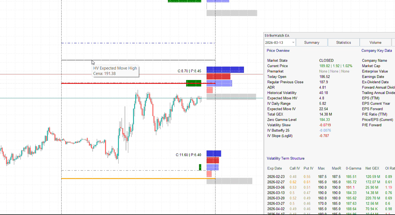
StrikeWatch EA plots the Expected Move directly on your MetaTrader 5 chart, eliminating the need for manual calculation or chain analysis. The full IV context that drives the EM calculation — IV Rank, IV Percentile, and the live IV–HV spread — is available in the Summary Surface module, described in the IV vs. HV guide. For the complete three-dimensional volatility surface that connects EM to skew and term structure, see the IV Surface framework.
- 1-SD and 2-SD Horizontal Lines: The Expected Move bounds are plotted as dynamic horizontal lines on your price chart, updated in real time as IV changes. The 1-SD lines (68% probability range) define the standard credit spread boundary. The 2-SD lines (95% range) define the extreme tail boundary and natural wing placement for wide condors.
- Automatic DTE Matching: The EM calculation automatically uses the nearest relevant expiration, so the bounds you see always correspond to the most actionable time frame for the current session.
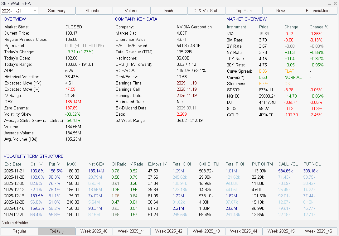
- On-Chart HUD Integration: The Expected Move values are displayed numerically in the StrikeWatch HUD alongside Max Pain, ZGL, and IV Rank — giving you the complete structural and probabilistic picture in a single glance without leaving your chart.
- GEX + EM Confluence Detection: When the highest positive-GEX strike falls within the EM bounds and aligns with a high-scoring strike wall, StrikeWatch EA surfaces this overlap in the OI/Volume Statistics module. This confluence is the ideal environment for iron condor placement: sell the EM bounds with dealer mechanical defense at the center — the double conviction scenario described in Section 6.
The Expected Move is IV translated into price. The formula — Stock Price × IV × √(DTE/365) — converts annualized implied volatility into the 1-SD (68%) probabilistic range for any expiration. Higher IV or more time = wider EM.
The ATM straddle price ≈ the Expected Move. No calculation required — read EM directly from the chain. Multiply by 0.85 for a precise 1-SD estimate. This is the professional floor shortcut for earnings and event trades.
EM defines probable vs. improbable outcomes. Credit strategies profit inside the EM; long-vol strategies profit outside it. The choice between them is a direct bet on whether IV is fairly priced relative to future realized volatility.
1-SD EM boundary at Delta ~0.16 = 84% probability OTM. This is the standard professional short-strike placement for iron condors — a position with roughly 2:1 edge on win rate before accounting for credit received vs. risk defined.
EM + Strike Wall score = structural conviction. A 1-SD boundary with a Wall score of 3–4/4 is a mechanical and probabilistic anchor. A boundary with a score of 1/4 is a statistical estimate only. Always cross-reference before placing a short strike.
GEX regime amplifies or undermines EM reliability. Positive gamma (above the ZGL) compresses realized ranges — EM bounds more likely to hold. Negative gamma amplifies moves — EM breaches are more frequent and more violent than the 32% theoretical rate.