What Is Historical Volatility?
Historical Volatility (HV) — also called Realized Volatility (RV) or Statistical Volatility (SV) — measures how much an asset's price has actually moved over a defined past period. It is a backward-looking, purely empirical calculation: you take the log returns of the closing prices over N days, compute their standard deviation, and annualize the result.
HVN = σ(log returns over N days) × √252
— Where √252 is the annualization factor for daily returns (252 trading days per year). Common lookback windows: HV10 (10-day), HV20, HV30, HV60, HV252 (1-year).
HV Across Lookback Windows
Different lookback windows answer different questions. HV10 is reactive — it captures the most recent burst of realized movement and is the most sensitive to short-term volatility spikes. HV20 and HV30 are the most commonly used by practitioners because they align with standard 30-day options cycles and balance responsiveness against noise. HV60 smooths out short-term distortions and reveals the medium-term volatility regime. HV252 represents the full-year baseline — the broadest measure of the stock's "typical" movement.
| Window | Lookback | Most Useful For | Sensitivity |
|---|---|---|---|
| HV10 | 10 trading days (~2 weeks) | Detecting recent volatility acceleration; 0DTE context | Very high — reacts to individual sessions |
| HV20 | 20 trading days (~1 month) | Comparing to front-month IV; VRP assessment | High — standard short-term benchmark |
| HV30 | 30 trading days | Primary VRP comparison window for 30-DTE options | Moderate — industry standard for VRP |
| HV60 | 60 trading days (~3 months) | Medium-term regime identification | Low — filters short-term noise |
| HV252 | 252 trading days (1 year) | Annual baseline; IVR/IVP denominator context | Very low — long-term structural view |
What HV Cannot Tell You
HV is not a forecast — it describes the past. A stock with HV20 = 35% has moved with an annualized standard deviation of 35% over the last 20 trading sessions. Whether it will continue to move that way is a separate question entirely — and that is precisely where Implied Volatility enters the picture. Using HV as a forward predictor without checking the current IV level is one of the most common errors in volatility analysis: past movement does not determine future option pricing; the market's current expectations do.
What Is Implied Volatility?
Implied Volatility (IV) is the volatility value that, when plugged into an options pricing model (typically Black-Scholes), produces the option's current market price. It is extracted from the market price rather than calculated from historical data — making it a forward-looking, market-consensus forecast of future realized volatility over the option's remaining life.
IV as a Reverse Calculation
IV is not something you observe directly in the market. You observe the option's bid-ask midpoint, and then you solve the pricing equation in reverse to find the volatility input that would justify that price. All other inputs — stock price, strike price, time to expiration, interest rate — are known. Volatility is the only unknown, and the market's current option price is the answer. This process is called implied volatility extraction.
This is why IV is sometimes described as the options market's collective "vote" on how much the underlying will move before expiration. If a large number of participants are willing to pay higher prices for options, IV rises — regardless of what HV says. IV is a price first, a forecast second. Understanding this distinction is critical: Vega — the Greek measuring an option's sensitivity to IV changes — is the direct channel through which IV affects your P&L on every options position you hold.
IV as a Probability Distribution
More precisely, IV represents the annualized standard deviation of log returns that the market is pricing into option contracts. An IV of 30% for a $200 stock implies the market assigns roughly a 68% probability that the stock will be between $140 and $260 one year from now — a ±30% range. For shorter time horizons, this range scales by the square root of the time fraction. This is the mathematical link between IV and the Expected Move — the practical output every options trader uses daily.
HV looks backward — it measures what the stock did.
IV looks forward — it measures what option buyers and sellers collectively
expect the stock to do. More precisely: it measures the price of uncertainty,
which includes both expected move and a risk premium paid to option sellers.
The IV–HV Spread: The Volatility Risk Premium
The difference between Implied Volatility and Historical Volatility is called the Volatility Risk Premium (VRP) or the IV–HV spread. It is one of the most persistent and exploitable structural edges in the entire options market.
Empirically, IV is almost always higher than subsequent realized volatility. Across all major equity indices and most liquid single stocks, the average IV overstates realized volatility by 2–5 volatility points over rolling 30-day windows. This premium exists because option buyers are willing to pay above fair value for insurance — and option sellers (primarily dealers and professional desks) harvest this premium systematically as their primary source of edge. For the VRP measured at the index level using the VIX, see the VIX Guide.
Reading the Spread Direction
The direction and magnitude of the IV–HV spread has direct, actionable implications for strategy selection:
| IV vs. HV | Spread | Market Interpretation | Options Strategy Implication |
|---|---|---|---|
| IV ≫ HV (IV much higher) | Large positive | Options are expensive; market expects a big move that hasn't materialized yet | Sell premium — short straddle, iron condor, covered calls |
| IV > HV (moderate) | Positive | Normal risk premium — options fairly priced with slight overvaluation | Neutral — small edge to sellers; use spreads to define risk |
| IV ≈ HV | Near zero | Options priced at fair value relative to recent realized vol | Strategy selection driven by directional view, not vol edge |
| IV < HV (IV lower) | Negative | Options are cheap; market underestimates recent realized movement | Buy premium — long straddle, long options, calendar spreads |
| IV ≪ HV (IV much lower) | Large negative | Extreme complacency; often precedes a volatility event | High-conviction long vol — buy straddles, long vega positions |
Why the VRP Persists: The Insurance Premium Analogy
The VRP is not an arbitrage opportunity that will be competed away — it is the structural reward for bearing uncertainty. Option buyers are purchasing insurance against large adverse moves: they pay a premium above the mathematically fair value of that protection because the psychological and financial cost of being unhedged in a crash exceeds the ongoing cost of the premium. This is identical to how homeowners pay insurance premiums above actuarially fair rates because the catastrophic loss from an uninsured fire outweighs the ongoing premium cost.
The option seller — typically a dealer, hedge fund, or systematic income trader — accepts this premium in exchange for bearing the tail risk. The VRP is their systematic compensation. This is why premium-selling strategies (iron condors, short strangles, covered calls) have a positive expected return over time: they are not "picking up pennies in front of a steamroller" when executed with discipline — they are systematically harvesting a genuine, recurring market premium.
The Three Structural Pillars of VRP Persistence
What makes the VRP structural rather than opportunistic is the institutional demand architecture that sustains it. Three independent forces continuously replenish the premium — and none of them are price-sensitive:
- Regulatory mandates (Basel III, Solvency II): Banks and insurance companies operating under Basel III and Solvency II capital frameworks are required to hold assets that hedge against catastrophic market events. Options-based hedges are among the few instruments that provide the convex payoff profile required for regulatory compliance. This creates an inelastic, non-price-sensitive buyer of puts — regardless of how expensive they look on an IV basis. The institutional demand floor for downside protection does not disappear when the VRP looks stretched.
- Institutional hedging mandates (career risk): A fund manager buying protective puts is paying more than the actuarially fair value because the cost of not being hedged during a crash — career risk, fund redemptions, margin calls — far exceeds the cost of the premium. This behavioral asymmetry between the cost of overpaying for insurance and the cost of being unhedged is permanent and self-renewing. It is not a bias that rational markets will arbitrage away; it is rationally optimal behavior given the incentive structure of institutional asset management.
- Market maker supply constraints: Dealers who take the other side of institutional hedging demand cannot fully offset their exposure at all times. The VRP is partially compensation for the inventory risk they carry between hedging cycles — particularly on the downside tail, where gap risk cannot be continuously delta-hedged. The compensation demanded for bearing this unhedgeable residual risk is a persistent premium embedded in option prices that shows up directly in the IV–HV spread.
The result: implied volatility is permanently biased upward relative to what subsequently materializes, because the market is rationally pricing the cost of fear — and that cost is continuously replenished by regulatory and institutional structures that cannot change on short notice. Carr and Wu (2009) analyzed S&P 500 options data and confirmed that the VRP is economically large, negative on average for option buyers, and time-varying — but never zero over any sustained period.
The VRP exists and its structural foundations are durable — but harvesting it safely requires explicit regime filters, position-sizing rules, and non-negotiable kill-switches. For a complete quantitative framework covering universe construction (index vs. single-name), strategy selection (variance swaps to iron condors), entry/exit rules, drawdown controls, and an example SPX Iron Condor system ruleset, see the Systematic Short-Vol Strategies: A Quant Framework for Harvesting VRP.
Contextualizing IV: Rank and Percentile
Knowing that IV is "40%" is meaningless without historical context. For a stock like NVDA, 40% IV may represent historically low volatility. For a utility stock, it may be extreme. Two metrics normalize raw IV against a stock's own history: IV Rank (IVR) — which places current IV on a 0–100 scale within its 52-week high/low range — and IV Percentile (IVP) — which counts what percentage of the past 252 trading days had lower IV than today.
The two metrics can diverge dramatically after a volatility spike: a single extreme earnings event inflates the IVR denominator for up to 12 months, while IVP distributes that same event across all 252 observations — a 0.4% weight. Understanding when they agree, when they diverge, and which to trust in each scenario is the central skill of operational volatility screening. For the complete calculation mechanics, the four-combination divergence matrix, the triple-confirmation entry rule (IVR + IVP + VRP spread), and a five-step workflow with multi-stock examples (AAPL, NVDA, TSLA, MRNA, XOM), see the dedicated guide: IV Rank vs. IV Percentile: Screening Workflow and Divergence Guide.
IVR ≥ 30 + IVP ≥ 50 + IV exceeds HV by ≥ 5 points = triple-confirmed
premium-selling environment — the highest-conviction entry for income strategies.
IVR < 25 + IVP < 30 = both metrics confirm historically cheap options
— the structural entry for long-vol and debit spread strategies.
When IVR and IVP diverge by more than 30 points,
IVP is the more reliable signal — it reflects the true frequency
distribution of IV, not a denominator distorted by a single spike event.
The Volatility Term Structure
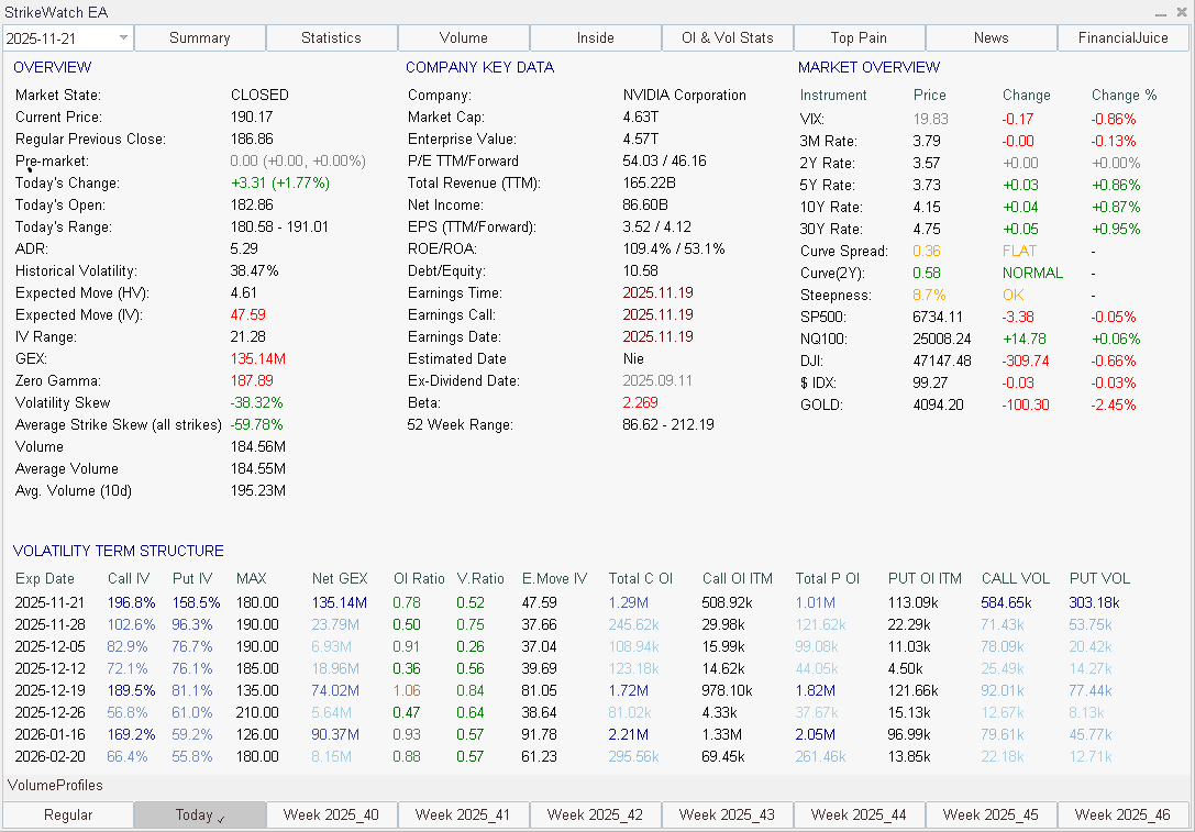
IV is not a single number — it varies across both strike price (the volatility smile/skew) and expiration date (the term structure). Under normal conditions, near-term IV is lower than longer-dated IV: the term structure slopes upward, reflecting greater uncertainty over longer time horizons. During stress events — earnings, macro catalysts, geopolitical shocks — the structure inverts: short-dated IV spikes above long-dated IV, signaling the market's perception of an imminent, discrete risk event.
The shape of the term structure directly amplifies or reduces the IV signal from IVR and IVP. An IVR of 60% in a normal contango structure is a clean premium-selling environment. The same IVR of 60% in a deeply inverted structure is a warning: do not sell short-dated premium without hedging vega exposure — the inversion signals unresolved risk that may not resolve before expiration. Persistent inversion beyond 3–5 sessions often precedes regime transitions toward negative gamma, where dealer hedging amplifies rather than absorbs directional moves.
The full term structure framework — contango vs. backwardation mechanics, calendar spread strategies, and the three-factor surface model that connects term structure to skew and volatility level — is covered in IV Surface: The Three-Factor Framework. That article is the domain hub integrating level, slope (term structure), and curvature (skew) into a single four-regime map — and is the recommended next step after completing this foundational guide.
From IV to Expected Move
The most direct practical output of the IV level is the Expected Move (EM) — the 1-standard-deviation price range the market prices in for a given expiration, derived directly from IV and time remaining. Every metric covered in this article feeds into EM: IVR tells you whether that probabilistic range is structurally cheap or expensive, and the IV–HV spread tells you whether the market's forecast has historically proven accurate relative to what the stock actually does.
For the complete EM formula, calculation examples across AAPL, TSLA, and SPX, the ATM straddle shortcut, strike-selection tables by EM boundary, and the interaction between EM bounds and GEX strike walls, see the dedicated Expected Move guide.
Translating IV Analysis Into Strategy Selection
With IV Rank, IV Percentile, the IV–HV spread, and the term structure shape in hand, strategy selection becomes a systematic, rules-based process rather than a discretionary judgment. The five core volatility environments and their corresponding strategies:
- IVR ≥ 50, IV ≫ HV, normal (contango) term structure: Classic premium-selling environment. The VRP is structurally elevated — options are expensive relative to recent realized movement, and the term structure offers no warning of imminent regime change. Sell defined-risk spreads (iron condor, short strangle with wings). Target short strikes at or beyond the 1-SD expected move. Manage positions at 50% of max profit or 21 DTE, whichever comes first. For 0DTE traders, IVR ≥ 50 combined with positive GEX is the highest-conviction sell-premium backdrop.
- IVR ≥ 70, IV ≫ HV, inverted term structure near earnings: Earnings IV-crush setup. The inversion is caused by the known catalyst — once earnings resolve, IV collapses rapidly and the term structure reverts to contango. Sell a short-dated straddle or iron condor the session before earnings, close the following morning after IV collapses. High win rate historically, but requires precise position sizing — the tail risk of a large earnings gap can exceed expected premium income. Never sell naked; always use defined-risk structures in this configuration.
- IVR < 25, IV ≈ HV or IV < HV, normal term structure: Premium-buying environment. Options are cheap relative to their historical range, and recent realized movement has matched or exceeded what IV was pricing. Long straddles, long strangles, or long calendar spreads favor the buyer — the edge comes from IV expanding back toward its historical mean (upside IV mean-reversion). This is also the environment where debit spreads offer the best risk/reward for directional trades, since the cost of buying options is structurally low.
- IVR < 20, sustained inverted term structure, price below ZGL: Extreme negative gamma regime with cheap options — rare but the highest-conviction long-vol setup available. Near-term IV is depressed despite the term structure inversion signaling unresolved structural risk, and dealer hedging (below the Zero Gamma Level) is amplifying rather than absorbing moves. Buy near-term options outright or construct ratio spreads. This specific combination has historically preceded the largest realized volatility expansions.
- IVR 30–50, IV–HV spread near zero: No structural vol edge in either direction. The market is pricing future movement approximately in line with what it has recently delivered. Strategy selection should be driven entirely by directional conviction or GEX/structural analysis from the Strike Wall framework. Avoid large net-vega positions in this environment; defined-risk vertical spreads that limit both vega and theta exposure are appropriate.
Common Misconceptions About IV
Volatility analysis is widely misunderstood even among experienced traders. These are the four most consequential errors:
- "High IV means the stock will move a lot." High IV means options are expensive relative to the stock's recent movement — it does not guarantee a large move will occur. High IV can persist or collapse without the underlying ever making the anticipated move. IV is a price set by supply and demand in the options market, not a reliable predictor of realized movement. A stock can have IVR of 80% and then spend the next month in a tight range — and the premium seller profits exactly from that scenario.
- "IV crush only happens after earnings." IV crush — a rapid decline in implied volatility — occurs whenever a pending uncertainty resolves: earnings, FOMC decisions, product launches, legal outcomes, macro data releases. Any identifiable event that drives IV inflation can cause a crush when it passes. Traders who sell premium before FOMC meetings or CPI prints (not just earnings) exploit the same IV-crush mechanics.
- "VIX is the only volatility measure that matters." VIX measures 30-day implied volatility on SPX options specifically. It is irrelevant for single-stock options, and even for index trading it must be combined with term structure analysis and the IV–HV spread to be actionable. A VIX of 20 in a normal contango term structure means something entirely different from a VIX of 20 in a deeply inverted structure with price below the ZGL. The VIX Guide covers the full index-level volatility framework, including VIX term structure and tradeable VIX products.
- "Selling premium is always the right strategy when IV is high." High IV is necessary but not sufficient for a premium-selling edge. If IV is high because the stock is about to make a very large move — a genuine fundamental catalyst where realized volatility will exceed implied — the seller will lose even from an elevated IV starting point. The edge in premium selling comes from the structural tendency of IV to overstate future realized volatility (the VRP), not from IV being high in absolute terms. Context — IVP, term structure, GEX regime — determines whether high IV is a selling opportunity or a warning signal.
Volatility Analysis Inside StrikeWatch EA
StrikeWatch EA centralizes every volatility metric covered in this article — from raw IV and HV to term structure visualization and the live IV–HV spread — in a single integrated interface inside MetaTrader 5:
- Live IV–HV Spread display: The Summary Surface module shows current IV (30-day ATM), HV20, HV30, and the live spread between them — updated on every data refresh. You always know whether you are in a VRP-rich premium-selling environment or a premium-buying environment without switching screens.
- IV Rank and IV Percentile side by side: Both IVR and IVP (trailing 252 days) are displayed simultaneously in the Summary Surface. Color coding instantly signals whether IV is historically elevated (green = premium-selling opportunity) or depressed (amber = premium-buying opportunity). When IVR and IVP diverge significantly, the display makes the discrepancy immediately visible — for the full diagnostic workflow to interpret that divergence, see IV Rank vs. IV Percentile: Screening Workflow and Divergence Guide.
- Volatility Term Structure heatmap: IV is visualized across up to 10 expiration dates as a multi-expiration curve — showing contango vs. inversion at a glance. The steepness of the curve and the location of kinks (earnings-related IV spikes in specific expirations) are immediately readable. For the full surface framework connecting term structure to skew and volatility level, see IV Surface: The Three-Factor Framework.
- Expected Move bounds on-chart: The 1-SD and 2-SD Expected Move boundaries for the nearest high-OI expiration are plotted as dynamic horizontal lines directly on your MT5 price chart — giving you structural context for every intraday decision without leaving the terminal. These bounds update in real time as IV changes throughout the session.
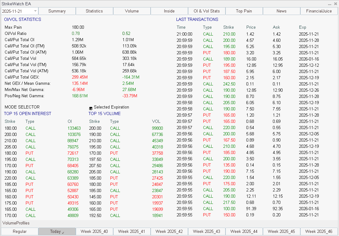
- Per-strike IV in OI/Volume Statistics: The OI/Volume module displays implied volatility for each of the Top 15 strikes by open interest — revealing the volatility smile and skew at a glance, and highlighting individual strikes with anomalous IV that may signal institutional positioning or structural repricing ahead of a catalyst.
HV measures the past; IV prices the future. The gap between them —
the Volatility Risk Premium — is one of the most persistent structural edges in options,
averaging 2–5 vol points of IV overstatement across major equity indices.
The VRP is structural, not cyclical. Three independent pillars sustain
it permanently: regulatory hedging mandates (Basel III / Solvency II), institutional
career-risk dynamics, and market maker inventory compensation. It cannot be arbitraged
away because its demand sources are non-price-sensitive.
The IV–HV spread determines strategy direction. IV ≫ HV = sell premium.
IV ≈ HV = trade direction, not volatility. IV ≪ HV = buy premium. The VRP persists
structurally because option buyers pay above fair value for insurance — and that excess
is the seller's systematic edge.
Always contextualize IV with IVR and IVP before selecting a strategy.
Raw IV is meaningless without historical normalization. For the complete two-metric
screening workflow, divergence matrix, and triple-confirmation entry rule, see
IV Rank vs. IV Percentile.
Term structure shape amplifies the IV signal. High IVR + normal
(contango) term structure = sell premium. High IVR + inverted term structure = sell
only with defined risk and reduced size. Persistent inversion is a regime warning, not
a selling opportunity.
The five-scenario framework is the systematic filter. IVR ≥ 50 + normal
structure → sell premium. IVR < 25 + IV ≤ HV → buy premium. IVR 30–50, spread near
zero → trade direction, not volatility. To extend this framework into the full
three-dimensional surface — integrating level, skew, and term structure into a single
regime map — see IV Surface:
The Three-Factor Framework.
To harvest the VRP systematically, not just understand it — including
entry/exit rules, drawdown management, and non-negotiable kill-switches — see
Systematic Short-Vol
Strategies: A Quant Framework for Harvesting VRP.